Magnetic Spectrum#
This notebook demonstrates the algorithm behind obtaining magnetic spectra.
Imports#
First we import the necessary libraries.
import time
from multiprocessing import set_start_method

from dotenv import dotenv_values
import matplotlib.pyplot as plt
import numpy as np
from matplotlib.collections import LineCollection
from matplotlib.colors import LogNorm, Normalize
from numpy import typing as npt
from phdhelper import mpl
from phdhelper.colours import sim as colours
from scipy import optimize
from tqdm import tqdm

import hybrid_jp as hj
import hybrid_jp.analysis as hja
Setting up the data#
Some parameters are set using environment variables. We load the deck first then the
.sdf files. This is so we can set the timestep, dt, which is defined in the deck
output. We also scale the magnetic field from its SI base units, Teslas \(T\), to
nanoTestlas \(nT\), and the same for the grid midpoints, \(m\rightarrow km\). Finally we
create a CentredShock object that holds the simulation data and has methods for
splitting the data held indside sdf files and grouping them into ‘chunks’, based on
distance upstream and downstream of the shock.
env = dotenv_values("../../../.env")
START, END = 20, 200
set_start_method("fork")
mpl.format()
data_folder = str(env["DATA_DIR"])
deck = hja.load_deck(data_dir=data_folder)
SDFs, fpaths = hja.load_sdfs_para(
    sdf_dir=data_folder,
    dt=deck.output.dt_snapshot,
    threads=7,
    start=START,
    stop=END,
)
for SDF in SDFs:
    SDF.mag *= 1e9  # Convert to nT
    SDF.mid_grid *= 1e-3  # Convert to km
cs = hja.CenteredShock(SDFs, deck)
100%|██████████| 181/181 [00:06<00:00, 29.36it/s]
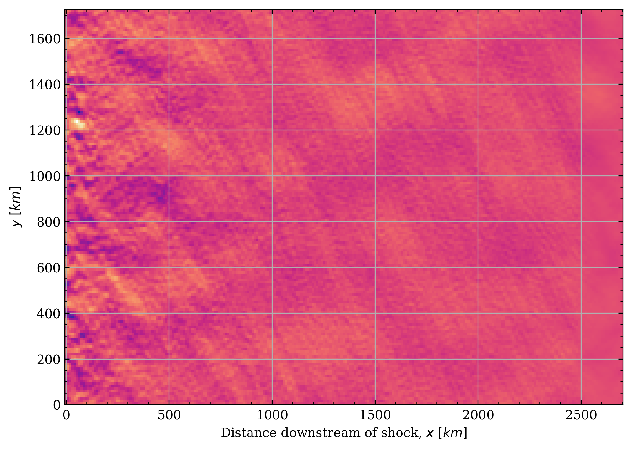
Getting values in a ‘frame’#
A ‘frame’ is an array of values at a given time and in a given chunk. The method
cs.get_qty_in_frame(func, chunk, t_idx) will slice the data returned by the function
func, at timestep t_idx, at chunk chunk. func must have the signature
Callable[[SDF], NDArray[np.float64]], i.e. it must take exactly one parameter, an
SDF object, and return an array. Below wer define the function get_bx() which
returns the \(b_x\) component from the SDF. This returns the whole array, which
get_qty_in_frame() then slices to the correct range in \(x\) to line up with the
specified chunk.
Important
the property cs.n_chunks must be set before calling most methods on cs, otherwise an
NChunksNotSetError will be raised.
Note
Alternatively, we could have obtained the meadian value of \(b_x\) in each cell, i.e. \(\left<b_x\right>_y\), using a function such as:
def get_median_bx(sdf: SDF) -> NDArray[np.float64]:
    return np.median(sdf.mag.bx, axis=1)
N_CHUNKS = 10
cs.n_chunks = N_CHUNKS
shock_chunk = cs.downstream_start_chunk


def get_bx(sdf: hj.sdf_files.SDF) -> npt.NDArray[np.float64]:
    return sdf.mag.bx


t = int(np.argmax(cs.valid_chunks[shock_chunk, :]))
qty, slc = cs.get_qty_in_frame(get_bx, shock_chunk, t)
plt.pcolormesh(
    cs.grid.x[slice(*slc)] - cs.grid.x[cs.get_x_offset_for_frame(shock_chunk, t)],
    cs.grid.y,
    qty.T,
)
plt.ylabel(r"$y\ [km]$")
plt.xlabel(r"Distance downstream of shock, $x\ [km]$")
plt.tight_layout()
plt.show()
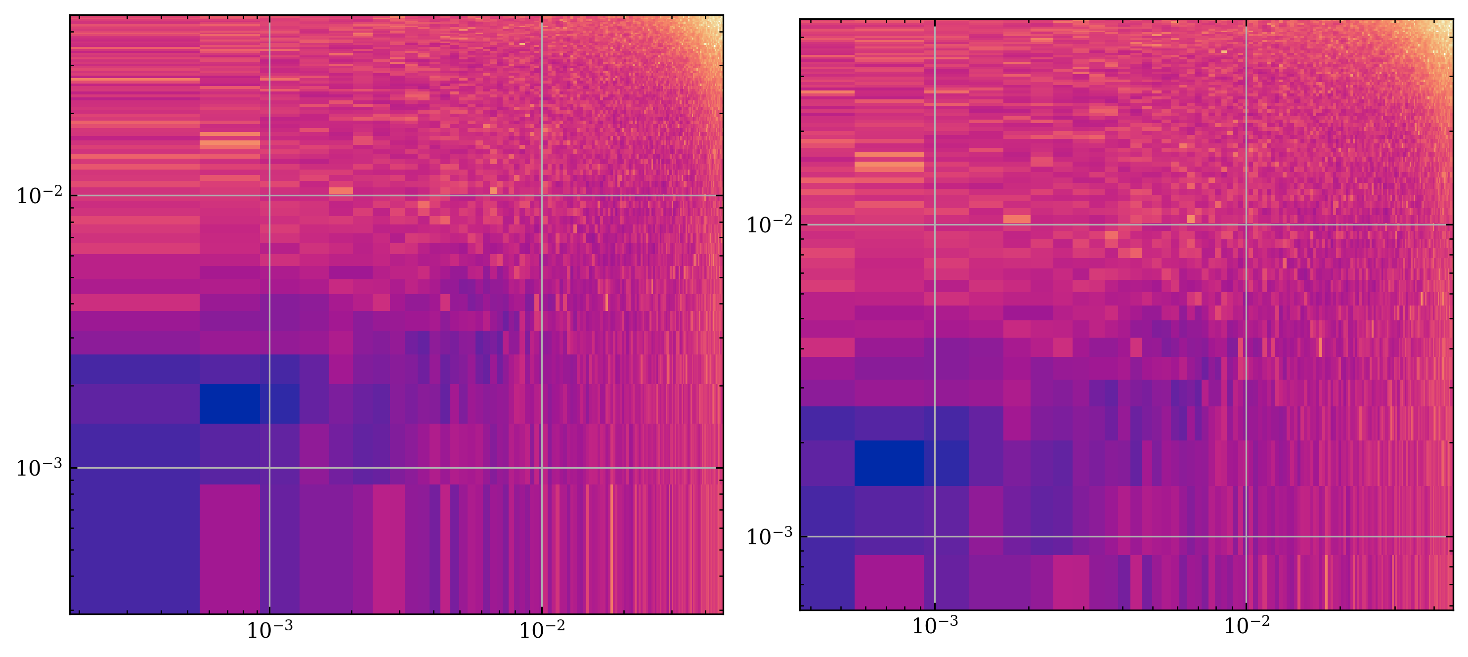
2D FFT and Subdivisions#
We now perform a 2d Fourier transform on the frame. Under the hood, this uses np.fft.fft2() function. Calling the function
bz_func = lambda x: x.mag.bz
bz = cs.get_qty_in_frame(bz_func, shock_chunk, t)[0]
pxy, kx, ky = hja.ffts.power_xy(bz, cs.dx, cs.dy)
axs: list[plt.Axes]
fig, axs = plt.subplots(1, 2, figsize=(10, 5))  # type: ignore
axs[0].pcolormesh(kx, ky, pxy.T, norm=LogNorm())
axs[0].set_yscale("log")
axs[0].set_xscale("log")
axs[0].set_aspect("equal")

pxy4, kx4, ky4 = hja.ffts.subdivide_repeat(4, pxy, kx, ky)
axs[1].pcolormesh(kx4, ky4, pxy4.T, norm=LogNorm())
axs[1].set_yscale("log")
axs[1].set_xscale("log")
axs[1].set_aspect("equal")
fig.tight_layout()
plt.show()
n_r_bins: int = 100
n_sub: int = 8
Pr4, kr = hja.ffts.radial_power(pxy, kx, ky, n_sub, n_r_bins)
kr = np.logspace(np.log10(kr[0]), np.log10(kr[-1]), n_r_bins)
print(Pr4.shape, kr.shape, n_r_bins * n_sub)

fig, ax = plt.subplots()  # type: ignore
ax.plot(kr, Pr4, c="k", ls="-")
ax.set_xscale("log")
ax.set_yscale("log")

fig.tight_layout()
plt.show()
(100,) (100,) 800
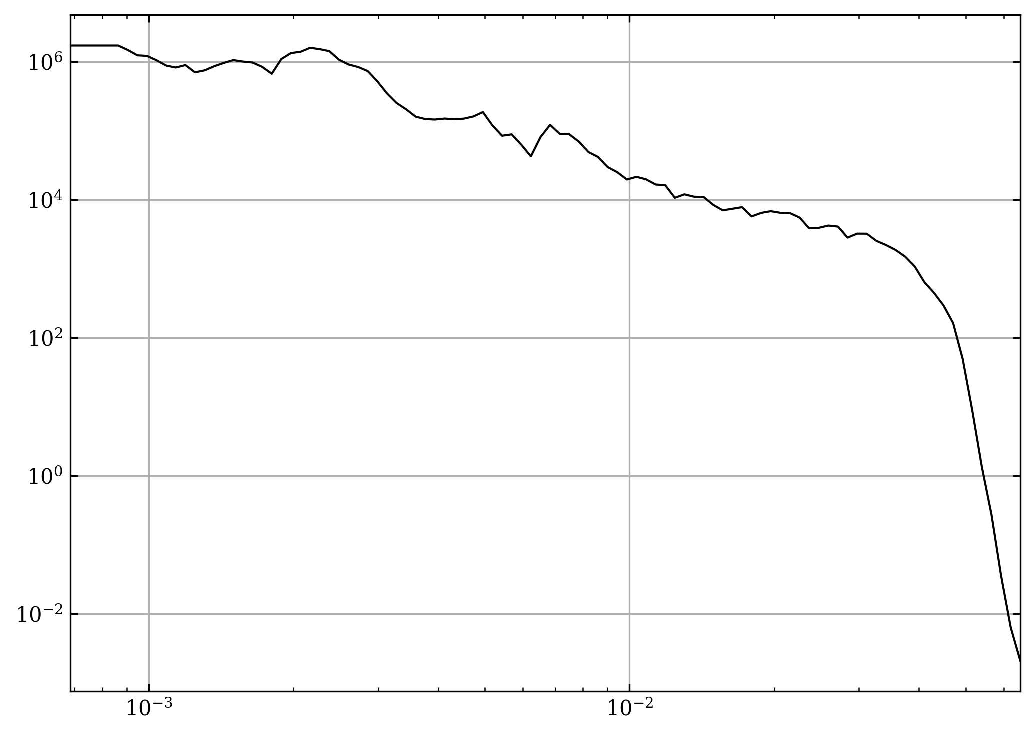
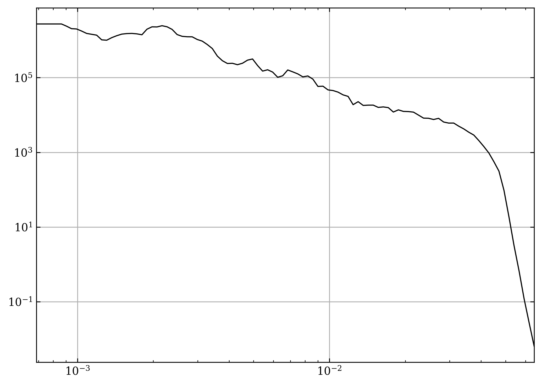
pr, kr = hja.frame_power(cs, shock_chunk, t, n_sub, n_r_bins)
fig, ax = plt.subplots()
ax.loglog(kr, pr, c="k", ls="-")
fig.tight_layout()
plt.show()
vc = cs.valid_chunks
val: list[list[int]] = [list(np.nonzero(vc[i, :])[0]) for i in range(vc.shape[0])]


def get_power_para(
    cs: hja.CenteredShock,
    val: list[list[int]],
    n_r_bins: int,
    n_sub: int,
):
    assert cs.n_chunks is not None

    kr = np.empty(n_r_bins)
    avg_pwr = np.empty((n_r_bins, cs.n_chunks))

    start_time = time.time()
    for i, v in enumerate(val):
        out = np.empty((n_r_bins, len(v)))
        for j, t in tqdm(enumerate(v), total=len(v), desc=f"Chunk {i}/{cs.n_chunks-1}"):
            out[:, j], kr = hja.frame_power(cs, i, t, n_sub, n_r_bins)
        avg_pwr[:, i] = out.mean(axis=1)

    end_time = time.time()
    print(f"Time taken: {end_time - start_time:.1f}s")

    return avg_pwr.T, kr


avg_pwr, kr = get_power_para(cs, val, n_r_bins, n_sub)
Chunk 0/9: 100%|██████████| 36/36 [00:04<00:00,  7.65it/s]
Chunk 1/9: 100%|██████████| 74/74 [00:09<00:00,  7.73it/s]
Chunk 2/9: 100%|██████████| 108/108 [00:13<00:00,  7.77it/s]
Chunk 3/9: 100%|██████████| 153/153 [00:19<00:00,  7.76it/s]
Chunk 4/9: 100%|██████████| 181/181 [00:23<00:00,  7.78it/s]
Chunk 5/9: 100%|██████████| 155/155 [00:19<00:00,  7.78it/s]
Chunk 6/9: 100%|██████████| 127/127 [00:16<00:00,  7.79it/s]
Chunk 7/9: 100%|██████████| 88/88 [00:11<00:00,  7.78it/s]
Chunk 8/9: 100%|██████████| 47/47 [00:06<00:00,  7.74it/s]
Chunk 9/9: 100%|██████████| 8/8 [00:01<00:00,  7.76it/s]
Time taken: 125.8s
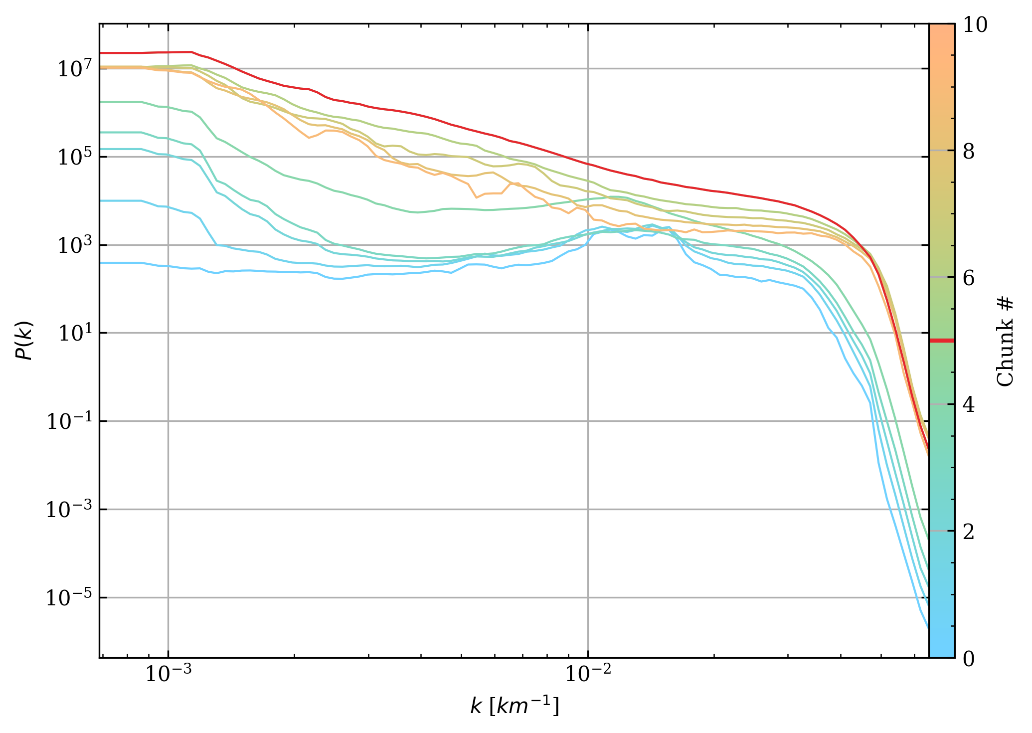
fig, axs = plt.subplots(1, 2, gridspec_kw=dict(width_ratios=[97, 3]))  # type: ignore
ax = axs[0]
cax = axs[1]


segments = np.array([np.stack([kr] * cs.n_chunks, axis=0), avg_pwr])
segments = np.moveaxis(segments, [0, 1, 2], [2, 0, 1])
norm = Normalize(vmin=0, vmax=cs.n_chunks)
lc = LineCollection(
    segments,  # type: ignore
    array=np.arange(cs.n_chunks),
    norm=norm,
    cmap=mpl.Cmaps.isoluminant,
)  # type: ignore
ax.add_collection(lc)  # type: ignore
ax.loglog(*segments[shock_chunk].T, c=colours.red())
ax.set_xscale("log")
ax.set_yscale("log")

fig.colorbar(lc, cax=cax, label="Chunk #")
cax.axhline(shock_chunk, c=colours.red(), lw=2)

ax.set_xlabel("$k$ [$km^{-1}$]")
ax.set_ylabel("$P(k)$")

fig.tight_layout()
fig.subplots_adjust(wspace=0)
plt.show()
# Slopes
def powerlaw(x, amplitude, exponent, constant):
    return amplitude * x**exponent + constant


def line(x, m, c):
    return m * x + c


min_x = 2e-3
max_x = 2e-2


def fitline(arr, min_x, max_x, func):
    # arr.shape = (n_chunks, 2) where 2 is (x, y)
    mask = (arr[:, 0] >= min_x) & (arr[:, 0] <= max_x)
    arr = np.log10(arr[mask, :])
    fit, _ = optimize.curve_fit(func, arr[:, 0], arr[:, 1])
    return fit


fig, ax = plt.subplots()
slopes = np.empty((cs.n_chunks, 2))
for i, s in enumerate(segments):
    slopes[i, :] = fitline(s, min_x, max_x, line)
    ax.plot(*np.log10(s).T, c="k", ls="-", lw=0.5)
    xr = np.log10(np.linspace(min_x, max_x, 2))
    ax.plot(xr, line(xr, *slopes[i, :]), c="r", ls="--")

plt.show()

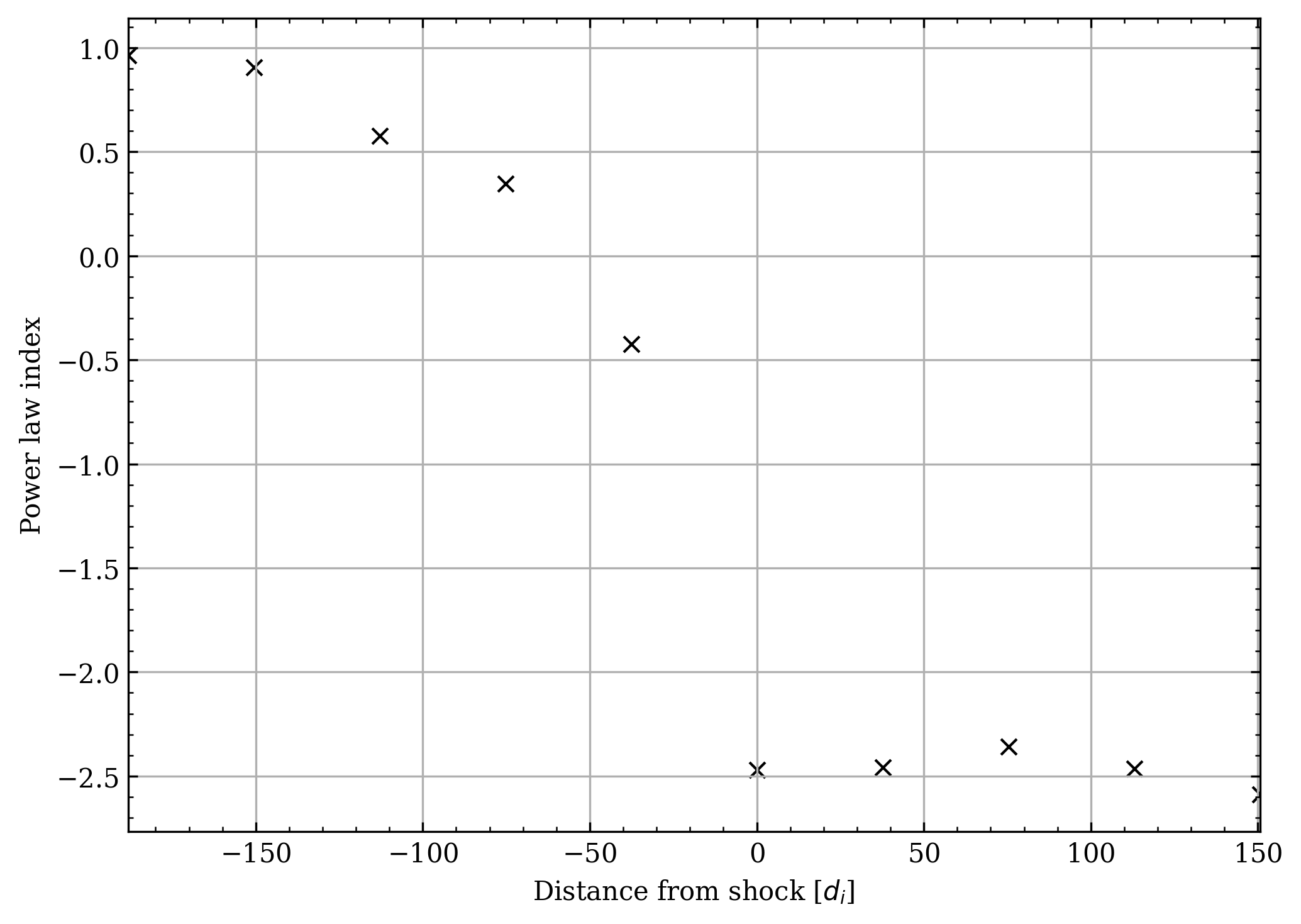
fig, ax = plt.subplots()

dists = (
    (np.arange(cs.n_chunks) - shock_chunk)
    * cs.dx
    * cs.chunk_i
    / (deck.constant.di * 1e-3)
)
ax.scatter(dists, slopes[:, 0], c="k", marker="x")  # type: ignore

ax.set_xlabel("Distance from shock [$d_i$]")
ax.set_ylabel("Power law index")


fig.tight_layout()
plt.show()